improved analysis of 9-bidder silent auction: friend's bid on San Francisco condo
After my last post, I commented that my analysis was obviously flawed, because it would lead to the conclusion the winning bidder had a 100% chance of winning. There were two obvious points of weakness in that analysis.
The first is I assumed the expectation value of the number of bidders was the number of bidders, not counting my friend. I don't count my friend because his presence wasn't random (I specifically picked this auction because he was there; I didn't pick it at random). However, that assumption is obviously just a guess. But lacking other information, it is the best I can do.
The next approximation I made was that the chance a random bidder was better than my friend's bid was the number of bidders who ranked better than my friend. This was 25%. This seemed a reasonable assumption, until I apply it to the case my friend wins the auction. In that case the result would be 0%. That's obviously wrong.
So what I assume is all bids can be mapped onto a uniform distribution from 0 to 1 (this isn't dollars, but rather a function of dollars). Then I generate a series of 9 random bids uniformly distributed from 0 to 1. I then take the 3rd ranked bid. The chance any given bid is better than this one is 1 - the value of the third-ranked bid. This might be 0.75. But it might be more or less.
Then using this probability I calculate the chance the friend would win the bid. If the value of the bid was 0.75, I get my previous estimate, which is 13.5%. But if the value were higher, for example 0.8, I'd get a larger chance, for example 20%.
I run this simulation 10 thousand times. In each case I pick a random set of 9 bids, I pick the third ranked one, I figure out the chance that third ranked bid would beat any random bid, and I calculate the chance that bid wins the auction considering all possible bidder turn-outs using Poisson statistics for the probability of that turn-out with the assumption the expectation value of the number of other bidders is 8.
Since I went through all this trouble, I did the calculation not just for the 3rd place bid out of 9, but for all possible places out of 9 from 1 to 9. Here's the result:
rank p
1    0.538398
2    0.286256
3    0.14854
4    0.075185
5    0.0370196
6    0.0174019
7    0.00752983
8    0.00308723
9    0.0011212
So the third place bidder had a 14.9% chance rather than 13.5% as I calculated last time. And the first-place bidder had a 53.8% chance, not 100% as I calculated last time.
A curious aspect of this is the sum is 111%. This is okay: it simply says that no matter what the place was on the current bid, just the fact the bidder participated gave him a chance, since there's always the chance the turnout would have been very small. There's no reason for the probabilities to sum to 1.
Of course, this ignores any information about how big the gaps were between bids. That would add additional information, but also additional complexity if that information were to be useful. I'd then need to add additional assumptions, for example on the probability distribution of bid amounts. I make no such assumptions here. This analysis is based only on bid rank and the assumption that there's no ties. Even in the case of dollar ties, there can be tie-breakers. I additionally assume there's no second round of bidding.
Here's a plot of those results, on a logarithmic scale:
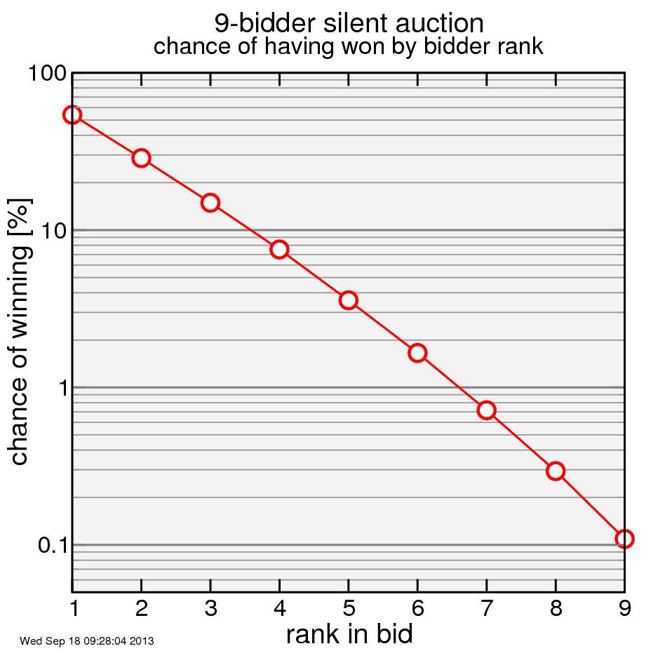
I then tried running for larger initial auctions. For the top bidders at these auctions, the winning chance becomes essentially independent of the number of people who were at the auction. The top bidder had around a 50% chance to win, the second bidder around 25%, the third 12.5, fourth 6.25%, etc: each successive bidder in the ranking had approximately half the chance of the bidder who ranked ahead, twice the chance of the bidder who ranked behind.
My friend was of the view that he'd lost: that he'd made a poor bid. But the whole process is stochastic. You've got to play the probabilities to maximize expected gain. And that analysis needs to recognize that the optimal probability of winning a given auction is not 100%, assuming price matters.


Comments